

How To Change The Scale Of A Scatter Plot In R
In this post, we will learn how to brand scatter plots using R and the package ggplot2.
More specifically, nosotros volition learn how to make scatter plots, change the size of the dots, modify the markers, the colors, and alter the number of ticks. Furthermore, we volition learn how to plot a trend line, add text, plot a distribution on a besprinkle plot, among other things. In the final department of the scatter plot in R tutorial, we volition acquire how to save plots in high resolution.
What is a Scatter Plot?
Earlier continuing this scatter plots in R tutorial, we will briefly talk over what a besprinkle plot is. This plot is a 2-dimensional (bivariate) data visualization that uses dots to represent the values collected, or measured, for two different variables.
That is, one of the variables is plotted along the 10-axis and the other plotted along the y-axis. For case, the scatter plot below, created in R, shows the relationship between speed and stopping distance of cars.
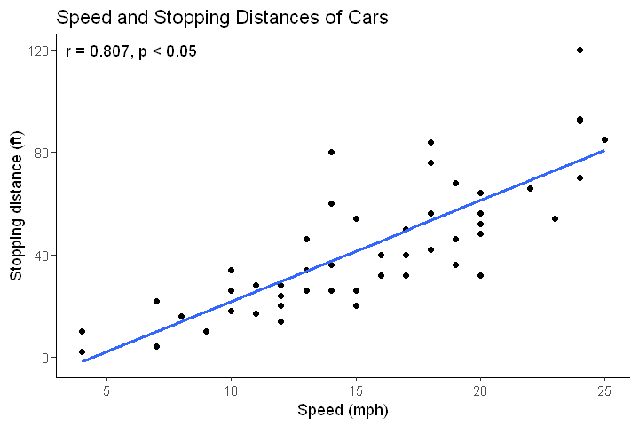
Note, in this scatter plot a trend line, too every bit the correlation between the ii variables, are added. Some other important attribute of the data analysis pipeline is doing descriptive statistics in R.
Required r-packages
In this scatter plot tutorial, we are going to utilise a number of different r-packages. Therefore, we demand to accept them installed before continuing. Now, the easiest style to get all of the packages is to install the tidyverse packages. Tidyverse is a corking package if you want to carry out information manipulation, visualization, among other things. For case, the packages yous get can be used to create dummy variables in R, select variables, and add a column or two columns to a dataframe.
How to Install R-packages
Here'south how to install the tidyverse package using the R command prompt using the install.packages() office,
install.packages(c("tidyverse", "GGally"))
Code language: R ( r ) If we only want to install the packages used in this besprinkle plot tutorial this is, of course, possible.
to.install <- c("magittr", "purrr", "ggplot2", "dplyr", "broom", "GGally") install.packages(to.install)
Lawmaking linguistic communication: R ( r ) In the more than recent postal service, y'all can learn about some useful functions and operators. For instance, if you need to generate a sequence of numbers in R you can use the seq() function. Some other useful operator is the %in% operator in R. This operator can be used for value matching.
How to Make a Besprinkle Plot in R
In this section, we will learn how to create a scatter plot using R statistical programming environment. In the beginning code chunk, below, nosotros print the dataset we start with; the mtcars dataset.
require(ggplot2) caput(mtcars)
Code linguistic communication: R ( r ) 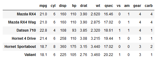
In nearly of the examples, in this besprinkle plot tutorial, we are going to apply available R datasets. Most of the fourth dimension, however, we will employ our ain dataset that can be stored in Excel, CSV, SPSS, or other formats. In the tutorial beneath, we volition learn how to read xlsx files in R.
- How to Read and Write Excel Files in R
Finally, earlier going on and creating the besprinkle plots with ggplot2 it is worth mentioning that you might want to practice some data munging, manipulation, and other tasks for you to start visualizing your data. For example, yous might want to remove a column from the R dataframe. Another matter, that you might want to exercise, is extracting timestamps, extracting year, or separating days from datetime.
How to use ggplot2 to Produce Scatter Plots in R
In this section, we will acquire how to make scattergraphs in R using ggplot2. First, we will have a quick look at the syntax used to create a simple scatter plot in R.
ggplot2 syntax to create a scatter plot in R
In the first ggplot2 scatter plot example, below, we will plot the variables wt (x-axis) and mpg (y-axis). This will give the states a simple scatter plot showing the relationship between these 2 variables.
Before going on and creating the first scatter plot in R we will briefly cover ggplot2 and the plot functions we are going to use. First, we start by using ggplot to create a plot object.
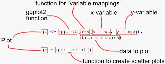
Inside of the ggplot() function, we're calling the aes() office that describes how variables in our information are mapped to visual properties. In this unproblematic besprinkle plot in R example, we just use the ten- and y-axis arguments and ggplot2 to put our variable wt on the 10-axis, and put mpg on the y-axis.
Finally, withal in the ggplot office, we tell ggplot2 to use the information mtcars. Next we're using geom_point() to add a layer. This function is what will make the dots and, thus, our scatter plot in R.
information(Salaries, package = "carData") gp <- ggplot(aes(x = wt, y = mpg), data = mtcars) gp + geom_point()
Code language: R ( r ) 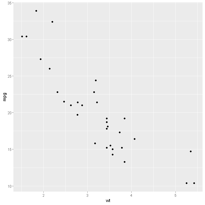
Here are more tutorials on data visualization in R:
- How to Create a Violin plot in R with ggplot2 and Customize it
How to Modify the Size of the Dots in a Scatter Plot in R
If we want to have the size of the dots represent ane of the variables this is possible. And so, how do y'all change the size of the dots in a ggplot2 plot? In the next example, we change the size of the dots using the size statement.
gp <- ggplot(aes(x = wt, y = mpg), data = mtcars) gp + geom_point(aes(size = four))
Code language: R ( r ) 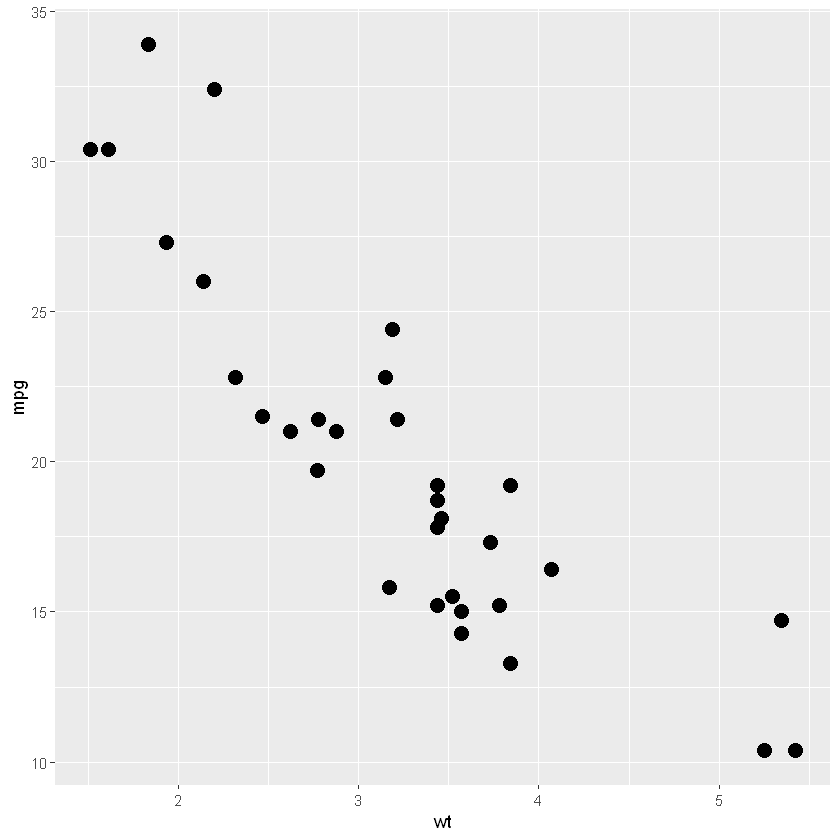
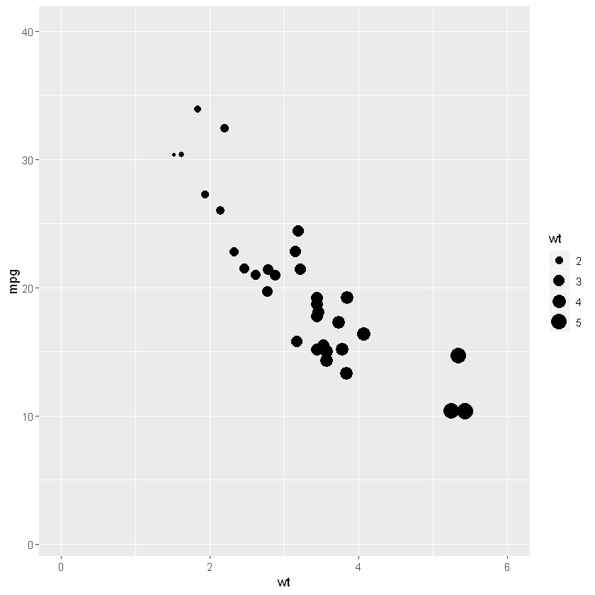
In the scatter plot case higher up, nosotros again used the aes() only added the size statement to the geom_point() function. When creating a scatter plot we can also change the size of the based on values from i of our columns. In the next example, nosotros are going to apply wt variable for the dot size:
Lawmaking linguistic communication: R ( r )
gp <- ggplot(aes(x = wt, y = mpg), data = mtcars) gp + geom_point(size = wt)
How to Change the Number of ticks using ggplot2
In the side by side scatter plot in R example, nosotros are going to learn how to change the ticks on the 10- axis and y-axis. That is, we are going to change the number of ticks on each centrality. This is done by adding two new layers to our R plot.
More specifically, to change the x-axis we apply the function scale_x_continuous , and to change the y-axis we apply the office scale_y_continuous. Furthermore, we use the arguments limits, which accept a vector, and nosotros can set the limits to change the ticks.
gp <- ggplot(aes(x = wt, y = mpg), data = mtcars) + geom_point() gp + scale_y_continuous(limits=c(1, forty)) + scale_x_continuous(limits=c(0, half-dozen))
Lawmaking language: R ( r ) 
In the adjacent scatter plot example, we are going to change the number of ticks on the x- and y-axis. To accomplish this, we add together the breaks statement to the above functions. Furthermore, we add the seq function to create a numeric vector.
gp + scale_y_continuous(limits=c(1, 35), breaks=seq(one, 35, 5)) + scale_x_continuous(limits=c(1.5, v.v), breaks=seq(1.5, 5.5, 1))
Lawmaking linguistic communication: R ( r ) Grouped Scatter Plot in R
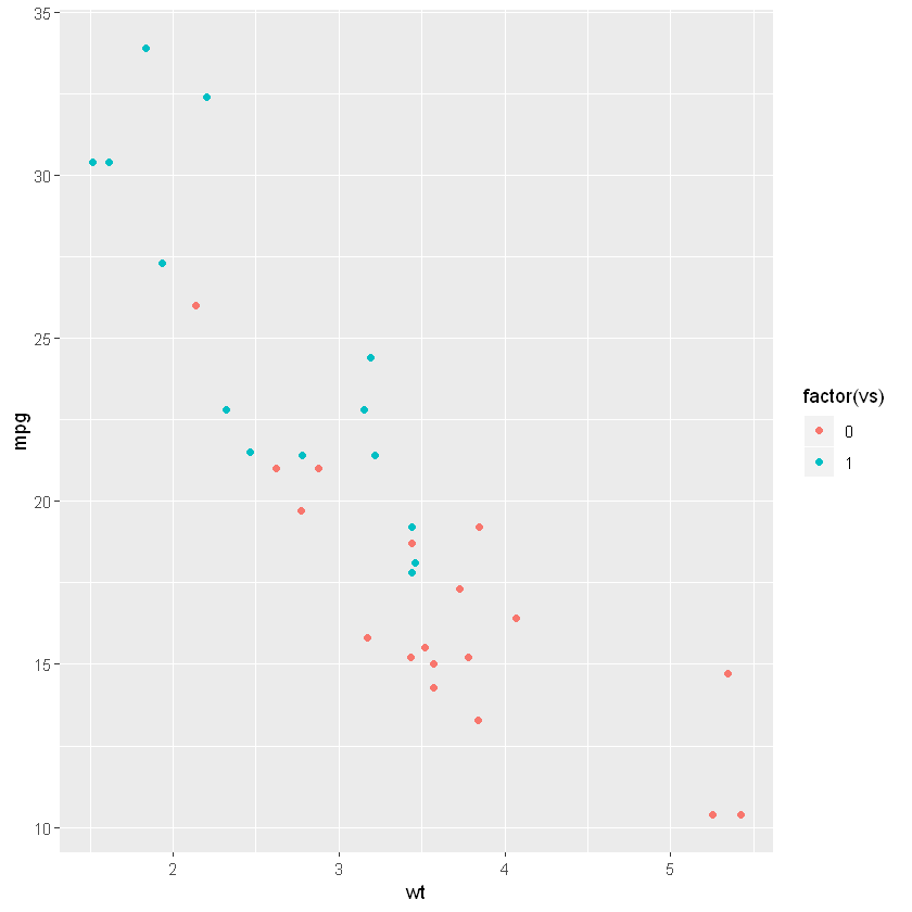
If nosotros have a categorical variable (i.e., a factor) and desire to group the dots in the scatter plot we use the colour argument. Note, that we apply the factor function to modify the variable vs to a factor.
Code language: R ( r )
gp <- ggplot(aes(ten=wt, y=mpg, color=gene(vs)), data=mtcars) gp + geom_point()
Alternatively, we can change the vs variable to a factor earlier creating the besprinkle plot in R. This is done using the every bit.factor function. This has the reward that the legend text will only say "vs". Here's how to modify a column to a factor in an R dataframe:
Code language: R ( r )
mtcars$vs <- equally.cistron(mtcars$vs) gp <-ggplot(aes(ten=wt, y=mpg, color=vs), information=mtcars) gp + geom_point()
Changing the Markers (the dots)
Now, one mode to alter the look of the markers is to use the shape statement. In the besprinkle plot in R, example beneath we are using a different dataset. Note, we are using the data part to load the Burt dataset from the package carData.
In the next, lines of code, we change the class variable to a cistron. Note that we are calculation thea aes() office in the geom_point() function. In the aes() function we are adding the color and shape arguments and add the grade column (the categorical variable). This way, our scatter plot is grouped by class both when it comes to the shape and the colors of the markers.
data(Burt, package = 'carData') Burt$class <- as.factor(Burt$class) gp <- ggplot(aes(x = IQbio, y = IQfoster), data = Burt) gp + geom_point(aes(color = class, shape = grade))
Lawmaking language: R ( r ) 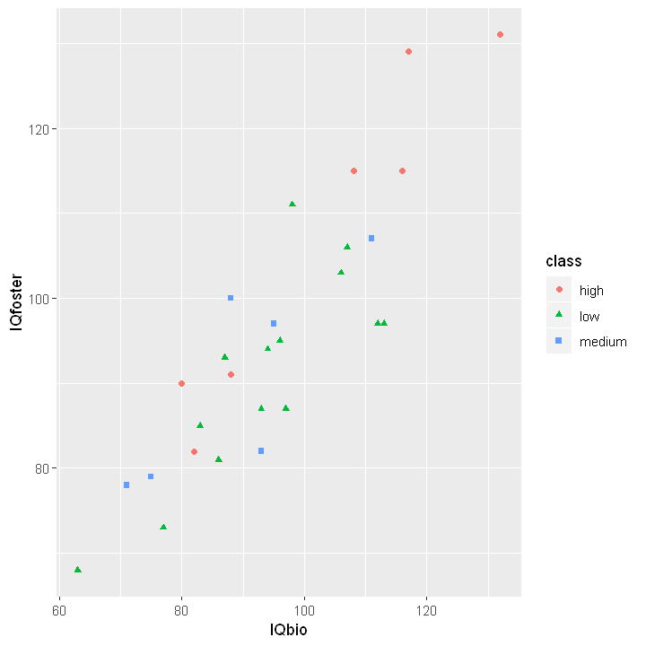
How to Add together a Trend Line to a Besprinkle Plot in R
In many cases, we are interested in the linear relationship between the 2 variables. For instance, we may continue by carrying out a regression analysis and want to illustrate the trend line on our scatter plot.
Luckily, this is quite easy using ggplot2; nosotros just utilise the geom_smooth() office and the method "lm". Finally, nosotros set the parameter se to Imitation.
gp <- ggplot(aes(x = IQbio, y = IQfoster), data = Burt) gp + geom_point(aes(color = grade, shape = form)) + geom_smooth(method = "lm", se = False)
Code linguistic communication: R ( r ) 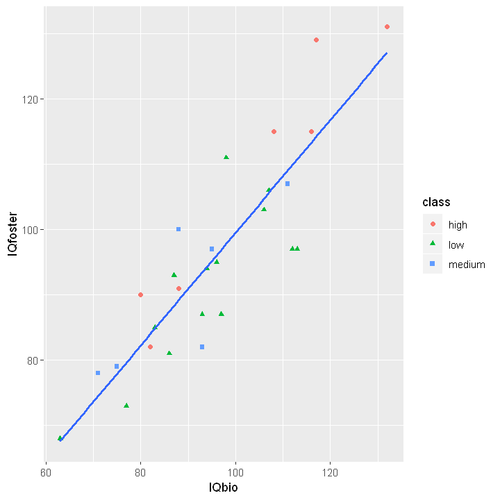
In the next besprinkle plot instance, we are going to add a regression line to the plot for each gene (category) also. Call up, nosotros just add together the colour and shape arguments to the geom_point() function:
gp + geom_point(aes(color = class, shape = form)) + geom_smooth(aes(color = form), method = "lm", se = FALSE)
Code linguistic communication: R ( r ) 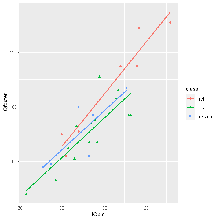
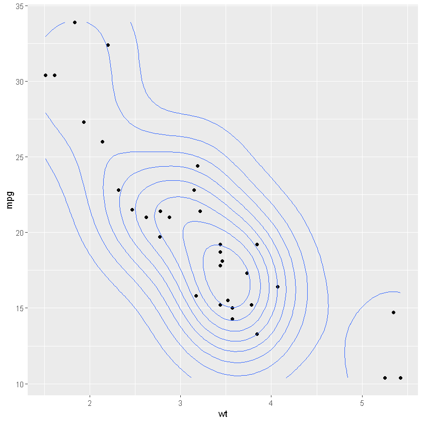
Bivariate Distribution on a Scatter plot
In the next besprinkle plot in R example, we are going to plot a bivariate distribution every bit on the plot. To reach this nosotros add together the layer using the geom_density2d() function.
Lawmaking linguistic communication: R ( r )
gp <- ggplot(aes(ten=wt, y=mpg), data=mtcars) gp + geom_point() + geom_density2d()
How to Add Text to Besprinkle Plot in R
In this section, we are going to carry out a correlation assay using R, extract the r– and p-values, and later learn how to add this as text to our scatter plot.
Here, we will use two additional packages and you tin, of course, bear out your correlation assay in R without these packages. The packages we are going to use hither are dplyr, and broom.
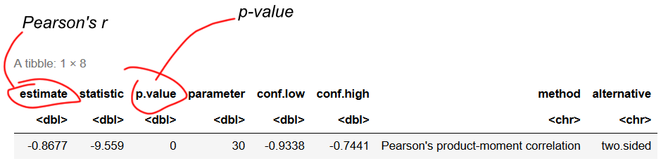
require(dplyr) require(broom) corr <- mtcars %$% cor.examination(mpg, wt) %>% tidy %>% mutate_if(is.numeric, round, 4) corr
Code linguistic communication: JavaScript ( javascript ) In the code chunk, above, nosotros are using the pipe functions %$% and %>%, cor.test() to carry out the correlation analysis between mpg and wt, and tidy() convert the result into a table format.
Finally, in the pipeline, we utilize the mutate_if with the is.numeric and round functions inside. The is.numeric part is used to brand sure the round office is only applied on numeric values.
The resulting table will have the values nosotros need, likewise as confidence interval, t-value (statistic), what method we used, and whether nosotros used a two sided or one sided examination:
Now that nosotros have our correlation results nosotros can extract the r- and p-values and create a graphic symbol vector. In the next code chunk, we use the paste0 and paste functions to do this. Furthermore, nosotros are using the ifelse function to print the total p-value if information technology'due south larger than 0.01.
text <- paste0('r = ', corr$judge, ', ', ifelse(corr$p.value <= 0, 'p < 0.05', paste('p = ', corr$p.value)) ) text
Code language: R ( r ) Adding Text to a Plot in R
It's time to put everything together. In this scatter plot with R example, nosotros are going to utilize the annotate function. When we use the annotate function, we utilise the 10 and y parameters for the positioning of the text and the label parameter is where we use our graphic symbol vector, text. Put only, we added a new layer to the ggplot2, with our text.
gp <- ggplot(aes(x = wt, y = mpg), data = mtcars) gp + geom_point() + geom_smooth(method = "lm", se = FALSE) + annotate('text', x = 4.5, y = 35, label=text)
Code language: R ( r ) 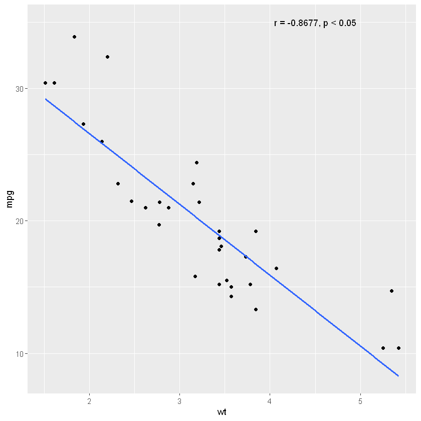
Now, what if we wanna plot correlations by group on a scatter plot in R? Well, in the next code chunk we are going to use the tidyr and purrr packages, equally well.
As this example is somewhat more than complex, compared to the previous i, we are not going into detail of what is happening. However, we utilise the pipe, %>%, over again. The nest role, here, is used to go the dataset grouped past course. More than specifically, it creates smaller dataframes (past course) within our dataframe.
Now, after we have practical the nest role, nosotros use mutate and create a column, within the new dataframe we are creating. We apply the map function where we carry out the correlation analysis on each dataframe (e.yard., by grade). Furthermore, we are using map_dbl function twice, to extract the p- and r-values. Finally, the mutate_if is, over again, used to round the numeric values and select will select the columns we want.
require(tidyr) crave(purrr) data(Burt, bundle = 'carData') corr <- Burt %>% group_by(form) %>% nest() %>% mutate(Cor = map(data, ~ cor.examination(.$IQbio, .$IQfoster)), p = map_dbl(Cor, 'p.value'), est = map_dbl(Cor, 'judge') ) %>% mutate_if(is.numeric, circular, 4) %>% select(course, p, est, Cor) text <- corr %>% mutate( text = paste0('r = ', est, ', ', ifelse(p <= 0.01, 'p < 0.05', paste('p = ', p))))
Lawmaking language: R ( r ) Learn more about selecting columns in the more recent post Select Columns in R past Name, Alphabetize, Letters, & Certain Words with dplyr.
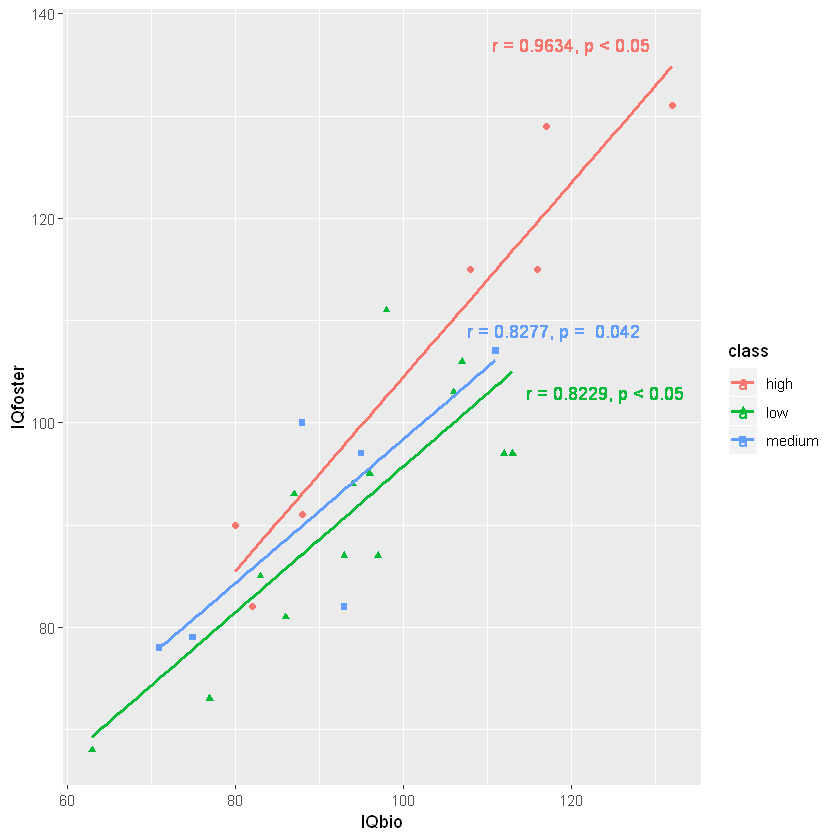
Note, the text (character vector) is, like in the previous case, created using paste0 and paste. In the scatter plot using R example, below, we are going to utilise the function geom_text() to add text.
Burt$grade <- equally.factor(Burt$grade) gp <- ggplot(aes(x = IQbio, y = IQfoster), data = Burt) + geom_point(aes(colour = class, shape = grade)) corrp <- gp + geom_point(aes(color = class, shape=course)) geom_smooth(aes(colour = class), method = "lm", se = Fake) + geom_text(aes(x = 120, y = 137, colour="loftier", label=subset(text, course == "high")$text)) + geom_text(aes(ten = 118, y = 109, color="medium", label=subset(text, class == "medium")$text)) + geom_text(aes(x = 124, y = 103, color="low", label=subset(text, class == "depression")$text)) corrp
Code linguistic communication: R ( r ) Now, in the lawmaking clamper above, we utilise the aes() function inside the geom_text part. Hither, we use the ten and y arguments for coordinate, color (set to each form), and characterization to set the text. Note, that we use the subset() function to make a subset of the text table with each form and we select the text by using the $ operator and the column name (text). The resulting scatter plot looks like this:
How to Style a Besprinkle plot in R
In this section, we are going to larn how to modify the grey background of the ggplot2 besprinkle plot to white. We are also going to learn how to add lines to the x- and y-axis, go remove the filigree, remove the legend title, and keys.
At present, to achieve this we add 3 more than layers to the above plot. First, we apply the part theme_bw() to get a dark-light-themed plot. After this, nosotros are going to make the scatter plot in blackness and grey colors using the scale_colour_grey() function. Finally, we add a theme layer using the function theme().
corrp + theme_bw() + scale_colour_grey() + theme(axis.line = element_line(colour = "blackness") ,plot.groundwork = element_blank() ,console.grid.major = element_blank() ,console.grid.minor = element_blank() ,strip.background = element_blank() ,console.edge = element_blank() ,legend.title=element_blank() ,legend.key = element_blank())
Lawmaking language: R ( r ) 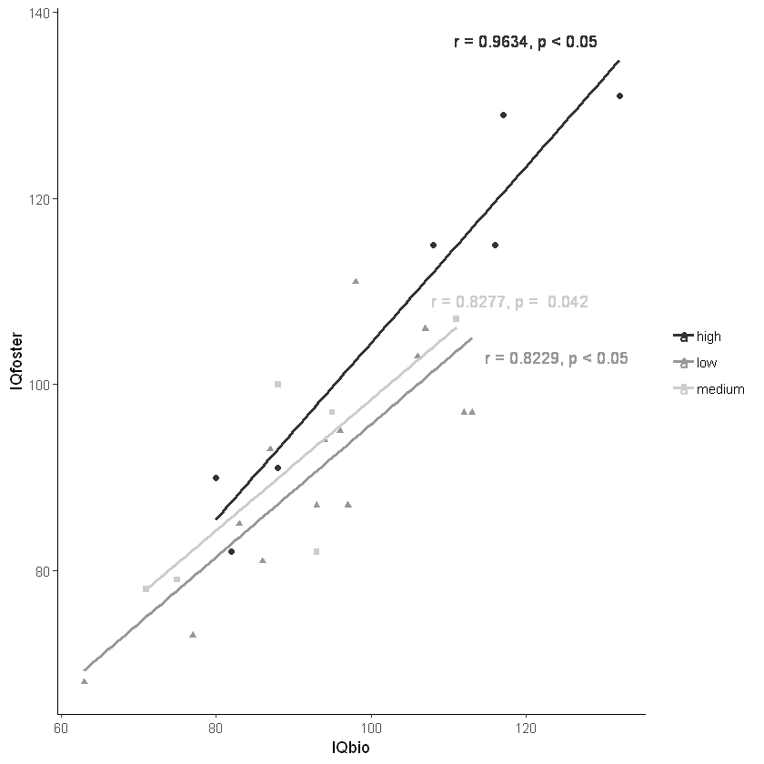
In the theme function, there are a lot of things going on and information technology may be easier to play effectually with removing the unlike elements. Notation, that the function element_blank() will make describe "zilch" at that particular parameter. For instance, plot.background = element_blank() will give the plot a blank (white) background.
How to Rotate the Axis of a scatter plot using Ggplot2
In this section, we are going to create a scatter plot with R and rotate the x-axis labels.
information(Salaries, package = "carData") Salaries$rank <- as.gene(Salaries$rank) gp <- ggplot(aes(ten = salary, y = yrs.since.phd), data = Salaries) + geom_point(aes(color = rank, shape = rank)) + geom_smooth(method = "lm") + scale_y_continuous(limits = c(0, lx)) + scale_x_continuous(limits = c(50000, 240000), breaks = seq(50000, 240000, by = 10000))
Code language: R ( r ) Now, as we have ready the x-ticks to be every 10000 we will become a scatter plot in which nosotros cannot read the axis labels. To accomplish this, we add together a theme layer using the theme() role. Here we utilise the axis.text.ten and employ the function element_text(). Inside the later function we ready the bending-argument to xc to rotate the text ninety degrees
gp + theme(axis.text.ten = element_text(bending = 90, hjust = 1))
Code language: R ( r ) 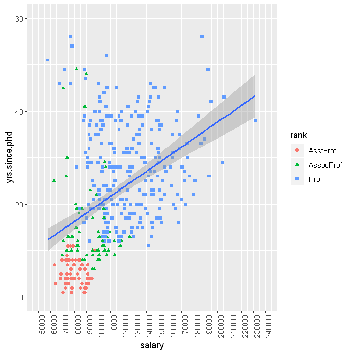
Pairplot in R: Scatterplot + Histogram
In the last department, earlier learning how to save high-resolution Figures in R, we are going to use create a pairplot using the package GGally. More specifically, we are going to create a scatter plot as well as histograms for pairs of variables in the dataset mtcars.
require(GGally) cols <- c('mpg', 'wt', 'hp', 'qsec') ggpairs(mtcars, columns = cols)
Code language: R ( r ) 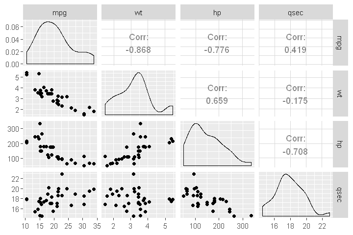
Saving a High Resolution Plot in R
Now that we know how to create besprinkle plots in R, we are going to learn how to salvage the pltos in high resuolution. In this section, we are going to learn how to salvage ggplot2 plots as PDF and TIFF files.
For instance, if nosotros are planning to apply the scatter plots nosotros created in R, we need to save the them to a loftier resolution file. In the final R code examples, we will learn how to save a high resolution image using R.
First, nosotros create a new besprinkle plot using R and we use most of the functions that we have used in the previous examples.
data(Salaries, parcel = "carData") gp <- ggplot(aes(10=yrs.since.phd, y=salary), data=Salaries) + geom_point() + geom_smooth(method = "lm", se = FALSE, colour="grey") + theme_bw() + theme(axis.line = element_line(colour = "blackness") ,plot.groundwork = element_blank() ,panel.filigree.major = element_blank() ,panel.grid.modest = element_blank() ,strip.groundwork = element_blank() ,panel.border = element_blank() ,legend.title=element_blank() ,fable.key = element_blank()) + xlab('Years since Ph.D.') + ylab('Bacon')
Code language: HTML, XML ( xml ) 2d, we use the ggsave() office to salvage the scatter plot. Note, in both examples here nosotros se the width and height in centimetres.
How to Salvage a Scatter Plot to PDF in R
At present, nosotros are ready to save the plot equally a .pdf file. In the lawmaking clamper, we use the device and set it to "pdf" too every bit giving the file a file proper name (ending with ".pdf").
ggsave("salaries_by_year_scatterplot.pdf", device = "pdf", width = 12, height = 8, units = "cm", dpi = 300)
Code linguistic communication: R ( r ) How to Save a Besprinkle Plot to TIFF in R
In the terminal code chunk, below, we are once more using the ggsave() function but change the device to "tiff" and the file ending to ".tiff".
ggsave("salaries_by_year_scatterplot.tiff", device = "tiff", width = 12, superlative = viii, units = "cm", dpi = 300)
Code language: R ( r ) Reproducible Data Visualization
Earlier concluding this scatter plot in R tutorial, we will briefly bear upon on the topic of reproducible research. Research is considered to be reproducible when other researchers can produce the exact results when having access to the original data, software, or lawmaking. This, of course, also ways that our plots need to exist reproducible. Learn how to create a fully reproducible surroundings in the Folder and R for reproducible science tutorial.
Conclusion
In this post, we take learned how to make besprinkle plots in R. Moreover, we have likewise learned how to:
- change the color, number of ticks, the markers, and rotate the centrality labels of ggplot2 plots
- save a high resolution, and print ready, image of a ggplot2 plot
Hither's a Jupyter notebook with the code used in this blog mail and hither is, the same notebook, on nbviewer.

Source: https://www.marsja.se/how-to-make-a-scatter-plot-in-r-with-ggplot2/
Posted by: smitharing1997.blogspot.com
0 Response to "How To Change The Scale Of A Scatter Plot In R"
Post a Comment